How AI Image Generation Works
None of its own. This is a stretch page and is not assessed as part of the machine learning topic. It explains generative AI, which A4.1.1 names as an application of machine learning, and connects to A4.2.3, A4.3.2, A4.3.8 and A4.3.9 (all HL) and to the ethics points A4.4.1 and A4.4.2. SL and HL students are both welcome. For assessed image-generation content, see the 2027 Case Study.
Three different ideas can make a computer produce a new image: two networks competing (GANs), compress-then-invent (variational autoencoders) and learning to undo noise (diffusion). Each section explains how the model trains and how it generates an image. The plain explanation comes first; the mathematical parts are labelled, so you can stop before them. The later sections cover text prompts, combinations of methods and ethical questions. For a shorter route, read the first paragraph of each method, then the ethics section. (Written July 2026 from sources dated 2022 to 2026. Claims about current systems carry a date.)
Table of Contents
- Reading an Image and Generating One Are Different Problems
- Method One: Two Networks in Competition (GANs)
- Method Two: Compress, Then Invent (Autoencoders and VAEs)
- Method Three: Learn to Undo Noise (Diffusion)
- Text Conditioning: How a Sentence Steers an Image
- A Fourth Family, in Outline: Flow-Based Models
- How the Methods Combine
- Comparing the Three Methods
- What About Video?
- Ethics: Who Made This Image?
- What This Page Leaves Out
- Where This Connects
Reading an Image and Generating One Are Different Problems
Stretch. Builds on A4.3.9, convolutional neural networks (HL). If you have met CNNs, you know how a computer reads an image; this page is the opposite direction, and it is not the same machinery run backwards.
An image classifier assigns a label to an input image. An image generator produces pixel values, often from random noise and sometimes with a prompt or input image to guide the result.
Generating is harder in one specific way: an image-generation task can have many acceptable outputs, so there is no single right answer to compare against. Most machine learning works by improving a measurable score, so the first job in generating anything is to choose a score that can be improved, such as how well generated images can be told apart from real ones, or how well added noise can be predicted. The three methods below are three different answers to that question, and asking “what score is being improved?” is a good way to tell them apart.
If you want the “reading” half fresh in your mind first, it is on Training and Evaluating a Model under CNNs (A4.3.9, in the syllabus).
Method One: Two Networks in Competition (GANs)
Stretch. Related to A4.3.2 (binary classification) and A4.3.8 (neural networks), both HL.
A generative adversarial network (GAN) is a competition between two networks with opposite jobs.
The generator produces images. At the start it is untrained, so it produces meaningless speckle.
The discriminator is shown a mix of real photographs (say, thousands of photos of real potted plants) and the generator’s output, and learns to say which is which. That is ordinary binary classification (sorting inputs into two categories), trained in the ordinary way: we know which images are real and which were generated, so every wrong call can be corrected. At the start the discriminator is untrained too, so it guesses. Neither network needs to be any good for training to begin.
The competition is the score that generation was missing:
- If the generator’s image fools the discriminator, that counts as success for the generator, and it adjusts to produce more like it.
- If the discriminator catches the fake, that is success for the discriminator and failure for the generator, which adjusts to avoid that kind of output.
Each network’s mistakes become the other’s training signal. A generator that is barely better than random can still sometimes fool a discriminator that is barely better than random, and each small win pushes both forward: a discriminator that gets harder to fool forces the generator to improve, which in turn gives the discriminator harder cases. When training goes well, the two improve together until the generated plants are hard for the discriminator, or a person, to tell from real ones. Training can also go wrong, though: it can fail to converge, as described below.
The two networks improve together. The generator is not given labelled examples of good images to copy: it learns only from the discriminator’s feedback on whether its images passed as real.
Try it: what is the easiest way to win? If the generator’s only goal is to fool the discriminator, what is the simplest strategy it could fall into? Think before revealing.
Show the failure this leads to
Find one image, or a small range of images, that reliably fools the discriminator, and produce it again and again. This failure is called mode collapse: the outputs cover only a small part of the variety in the training data instead of spreading across it. The failure comes from the incentive itself, not from a bug: the generator is rewarded for fooling the discriminator, not for variety. Follow-up question: what would you change in training so that repeating the same output stopped paying off?
When adversarial training goes wrong. In mode collapse, nothing malfunctions: the generator optimises the goal it was given, and the goal is not quite what anyone wanted. A badly chosen reward in reinforcement learning causes the same kind of problem. Two more failures matter, because training stability is part of evaluating this method:
- Failure to converge. Each network keeps reacting to the other’s latest changes, so training can oscillate rather than settle. Because the discriminator keeps changing, there is no single score that falls steadily the way a loss curve does in supervised training, so the loss values are harder to read as a measure of image quality.
- One side overpowering the other. A discriminator that gets too good too quickly rejects everything with complete confidence. The generator’s feedback collapses to “wrong” with no hint of which direction would be less wrong, and it stops improving.
Possible adjustments include changing the networks’ relative learning rates, limiting how quickly the discriminator learns and choosing a loss function that provides useful gradients to the generator. Managing this balance is one difficulty of adversarial training, and one reason to consider the other methods below.
For the assessed treatment of GANs, see the 2027 Case Study.
Method Two: Compress, Then Invent (Autoencoders and VAEs)
Stretch. Related to A4.2.3, dimensionality reduction (HL): an autoencoder learns a compact representation from which it reconstructs the input.
Start with a puzzle, before any theory.
Try it first: compress three numbers into one. Here are four rows of three numbers:
2,  4,   8
3,  9,  27
4, 16,  64
5, 25, 125
Replace each row with a single number, chosen so that someone who sees only your number can rebuild all three originals. Find the rule before revealing.
Show the rule and why it matters
Each row is a number, its square, and its cube. So the rows compress to 2, 3, 4 and 5, and anyone holding “3” can rebuild “3, 9, 27”.
The exercise illustrates four features of compression:
- Three values became one, and nothing was lost.
- To find the compression you had to find the pattern shared by all four rows: compressing the data well depended on understanding it.
- You inferred the rule from examples. An autoencoder also learns from examples, though it does so by adjusting numerical parameters.
- Real data may only approximately fit a pattern, so compression can lose some information. A real system rebuilds something close to the original rather than an exact copy, which is still useful.
Extension: can the same rule represent a fifth row, such as 4, 10, 19? Explain what information would be lost.
An autoencoder has two parts joined in the middle. The encoder takes the input (perhaps thousands of pixel values) and compresses it to a short list of numbers called the code. The decoder takes only the code and tries to rebuild the original. Training adjusts both parts to reduce the reconstruction error, which is the same task as the puzzle above: rebuild what went in after passing it through a narrow middle (a bottleneck).
Wide, narrow, wide: the encoder compresses the input into a code, and the decoder rebuilds it from that code. The set of possible codes forms the latent space (latent* means hidden: it is the middle representation, not anything visible in the image). Why train a network to output what you put in? To compress an image and still rebuild it, the network has to find the patterns in the data, so the code ends up holding meaningful information.*
A plain autoencoder is a compressor rather than a generator: it is trained to rebuild the inputs it is given. A variational autoencoder (VAE) adds one change that turns it into a generator: it also learns, and constrains, how the codes are spread through the latent space, so it knows where codes for real inputs tend to land. After training, the encoder can be set aside. Pick a point at random from that region and pass it through the decoder, and out comes a generated image in the style of the training data.
Sampling a code from the latent space and decoding it is the step that turns a compressor into a generator.
Method Three: Learn to Undo Noise (Diffusion)
Stretch. Related to A4.1.1, machine learning applications: as of 2026, diffusion is behind many widely used image-generation tools.
Diffusion is built on an asymmetry: destroying an image is easy, and creating one is hard. Diffusion models learn to reverse the easy direction.
Destroying an image takes no skill. Take every pixel, change its red, green and blue values by a small random amount (that random speckle is what noise means here), and repeat. After enough steps, any photograph becomes something like television static.
The trick is to train a network to run the easy direction backwards, one small step at a time:
- Training. Take a real photograph. Add a little noise, and keep the before-and-after pair. Add a little more, keep that pair too. Repeat until the image is pure static. Every adjacent pair is a training example: “this is what one step of damage looks like; learn to undo it.”
- Generating. Start from pure random static, which costs nothing to produce. Apply the trained undo-one-step network. Apply it again, and again, until an image emerges.
Why many small steps rather than one big jump? Undoing one small step of noise is a learnable task, because the image before the step is still mostly visible. Going from pure static to a photograph in a single jump gives the network almost nothing to work from. Training therefore uses examples at many different noise levels, so the network learns to denoise both slightly and heavily corrupted images, and generation repeats the small denoising step until an image forms.
The noise ladder. Each rightward step is trivial damage; the trained network learns only the small leftward step, and generation is that step repeated from pure static.
Two common questions:
- “So it recovers the original photo?” No. Generation starts from newly sampled static, not from a noisy version of a training photo, and the network produces a plausible image using the patterns it learned. That does not make every output original, though: diffusion models can memorise some training images and reproduce them closely; see Carlini et al. (2023). The difference between a plausible image and a copied one matters again in the ethics section.
- “Is the noise just any randomness?” Random, but not arbitrary. The nudges follow a stated spread (small changes likely, large ones rare), and the undo step is trained against exactly that spread.
Try it: add noise on paper. Draw a four-by-four grid, with the top two rows one colour and the bottom two another. Change each square’s colour slightly and randomly, then redraw. Ask a friend to work out the original pattern: after one step this is usually easy. Repeat the changes twenty times and ask again: by then very little of the pattern remains. That difference is why a diffusion model learns to undo noise in small steps, from many examples at different noise levels. (A bigger version: take one of your own photos, save five copies with more and more noise added in a photo editor, then view the sequence in reverse. The reversed sequence resembles what a diffusion model does when it generates an image.)
Finally, text enters. If every training photograph comes with a written description, the denoising network can also receive a representation of that text as it works. This conditioning steers generation from static towards an image that matches a description, such as “a lighthouse at sunset”, rather than towards any image at all. The next section explains how the words steer the image, and it is the more mathematical part of the page.
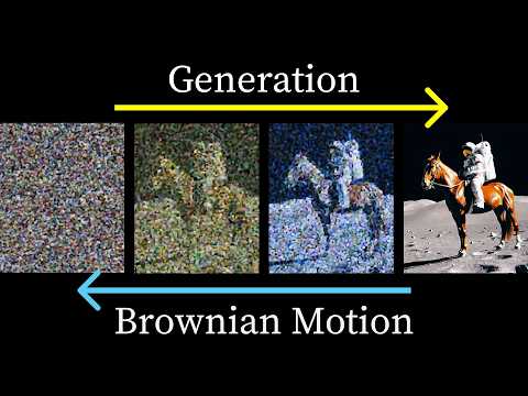
A visual explanation of diffusion, from 8:15. The full video is 37 minutes long and mathematical; its earlier part covers embeddings and how text steers the image, the ideas in the next section. The tools it names date from around 2022, so treat them as examples from that time; the mechanism it explains is the one described here.
Text Conditioning: How a Sentence Steers an Image
Stretch, and the advanced half of this page: the ideas are geometric and the sources are mathematical. Builds on A4.2.3 (a shared embedding space is a compact learned representation) and A4.3.2 (a classifier appears as a side effect). If this section is one layer too far, skip to the comparison: the rest of the page does not depend on it.
For text to steer image generation, text and images first have to be comparable at all. That is what CLIP provides (Contrastive Language-Image Pretraining). It is two encoders trained together: one turns an image into a vector (a list of numbers), the other turns a caption into a vector, and training pulls each matching image-and-caption pair close together while pushing mismatched pairs apart. That push-and-pull training is what “contrastive” means. Closeness is measured by cosine similarity, high when two vectors point the same way.
The result is one shared space holding both pictures and words, and it behaves like the word space on the language models page: directions carry meaning. The source demonstrates this with a hat; our version: take the vector for a portrait wearing sunglasses, subtract the vector for the same portrait without them, and the difference lands near the vector for the word “sunglasses”.
Pictures and captions in one space. The shared space also gives you a classifier: to label an image, compare its embedding with the embeddings of candidate captions and choose the highest-scoring match. This is nearest-match classification (A4.3.2) working on meaning rather than on pixels.
With the shared space in place, the steering machinery is three ideas stacked:
- Conditioning: feed the caption’s vector into each denoising step, so every removal of noise also moves the image towards one matching the description.
- Classifier-free guidance: run each step twice, once with the prompt and once without, take the difference between the two directions, and exaggerate it. The guidance strength setting controls the exaggeration: turned up, the output follows the prompt more forcefully (and, pushed too far, starts looking less natural).
- Negative prompts: the same arithmetic in reverse. Describe what you do not want, and subtract that direction.
For the full mathematical treatment, the Welch Labs video above covers CLIP from 3:37, cosine similarity from 5:36, the shared space and its directions from 6:24, conditioning from 26:41, guidance from 29:53 and negative prompts from 33:37.
A Fourth Family, in Outline: Flow-Based Models
Stretch. Related to A4.2.3 through the comparison between reversible transformations and compression that loses information.
The three methods above all accept losing information somewhere. A GAN never reconstructs anything. An autoencoder’s decoder lands close to the original rather than exactly on it. Diffusion destroys information on purpose every time it adds noise.
Flow-based models avoid that loss. They build the path from noise to image out of invertible transformations (steps that can each be exactly undone), so the chain runs in both directions: noise passed forward becomes an image, and an image passed backward recovers the noise it came from. The benefit is that, with suitable transformations, the model can calculate how likely a given image is under what it has learned about the data. The cost is design freedom: every step must be invertible, which restricts the operations the network can use. In short, reversibility is the idea, and exact likelihood in exchange for design freedom is the trade-off.
How the Methods Combine
Stretch. Image-generation systems can combine methods, for example by applying diffusion in an autoencoder’s latent space.
Diffusion as described above is expensive: every denoising step processes every pixel of a full-size image, and generation takes many steps. An autoencoder compresses an image into a much smaller code that keeps the important information. Latent diffusion puts the two together: run the denoising loop on that small code instead of on raw pixels, and decode to a full image only once, at the end. The expensive part now happens on something far smaller. Many text-to-image systems use this design (as of 2026), with a text encoder, such as one from the CLIP family described above, supplying the prompt. Adversarial training appears inside these hybrids too: a discriminator attached to the autoencoder’s decoder pushes its output to look realistic rather than only close to the original, which improves fine detail.
These methods can be combined in one system. Compare what each does well and where it could help in the process. For an assessed application, see the Hybrid Models page in the Case Study section.
Comparing the Three Methods
Stretch, connected to A4.3.10 (HL): complete the table to compare the methods for a particular task. For an extension, add a row for flow-based models.
Copy this table and complete it using the explanations above. For limitations not covered here, consult the linked case-study pages.
| What score is being improved? | How many networks? | One pass or many? | What does failure look like? | |
|---|---|---|---|---|
| GAN | ||||
| VAE | ||||
| Diffusion |
Compare your answers
- GAN: score = how often the generator fools the discriminator (the two networks have opposing objectives). Two networks. One generator pass produces an image. Failure: mode collapse (the outputs look alike), and training that fails to converge.
- VAE: score = how closely the decoder’s rebuild matches the original, plus keeping the codes evenly spread through the latent space (regularisation). One network in two halves, an encoder and a decoder. One decoder pass generates an image. Failure: not covered on this page.
- Diffusion: score = how well the network removes noise from a noisy image. One network, applied many times, so generation takes many passes. Failure: not covered on this page.
This page does not cover every failure, so some cells may stay empty. For more on limitations and evaluation, see Evaluating Models.
What About Video?
Stretch. Related to A4.4.1: moving images raise the same authorship and consent questions as still images, with higher stakes. The Welch Labs video shows pure noise becoming a moving scene (from 0:47). The basic idea is one you already have: diffusion, with the extra requirement of temporal consistency (objects and movement should stay coherent from one frame to the next). How that consistency is achieved is beyond this page. (Claim dated 2026.)
Ethics: Who Made This Image?
In the syllabus: A4.4.1 and A4.4.2 examine questions like these with the command term Discuss (consider different perspectives and support a conclusion), so read this section even if you skipped the mathematical ones.
Consider these questions about training data and generated images:
- Training data and consent. Image models are often trained on photographs and artwork collected from the web, including work by living artists who were not asked. Did the creators consent to this use, and how should they be credited or compensated? A model usually generates new images rather than retrieving stored ones, but it learned its abilities from that work: is that like an artist learning from others, or copying at industrial scale? Models can also memorise and reproduce some training images, which raises copyright and privacy concerns; see the research on diffusion-model memorisation. The same questions apply to language models trained on writers’ work.
- Plausible is not the same as real. A generator produces images that look like photographs of events that never happened. What happens to “seeing is believing” as evidence, in courtrooms, journalism and your own group chats?
- Who is the author? If you wrote the prompt, the company trained the model, and ten million photographers supplied the training data, whose image is it, and who is accountable when it causes harm?
The Welch Labs video discusses training data and authorship from 34:26. For accountability, consent and bias, continue to Ethics of Machine Learning.
What This Page Leaves Out
This page does not cover the following topics:
- Editing rather than generating: filling in part of an image, extending one, upscaling, style transfer.
- Evaluating generated images: see Evaluating Models in the Case Study section.
Where This Connects
- In the syllabus: What Machine Learning Is (A4.1.1: generative AI as an application; A4.1.2: why this all runs on parallel hardware).
- In the syllabus (HL): Training and Evaluating a Model for dimensionality reduction (A4.2.3, which an autoencoder performs), CNNs (A4.3.9, which read images rather than generate them) and neural networks generally (A4.3.8); Types of Learning for classification (A4.3.2, the discriminator’s job, and a use of the CLIP shared space).
- In the syllabus: Ethics of Machine Learning (A4.4.1) and Computing in Daily Life (A4.4.2) for the questions in the ethics section.
- Stretch: How Large Language Models Work uses the same embedding idea, where meaning is represented as position in a space; AI Beyond Machine Learning covers AI methods that work from rules and search rather than training.
- Assessed (Paper 1 Section B, 2027 cohort): the Case Study section covers image-generation techniques, GANs, diffusion, hybrid models, evaluation, and the ethics and law as examined material. This page is the conceptual background behind it.
Sources and dates for this page
Written July 2026, drawing on: Welch Labs, “But how do AI images and videos actually work?” (embedded above; its examples date from around 2022); CS50’s “Fundamentals of AI” lectures on computer vision and Generating (2026), which are long live recordings and so are linked rather than embedded; and Carlini et al., Extracting Training Data from Diffusion Models. All worked examples and diagrams on this page are original; the compression exercise uses different numbers and framing from any source. The linked 2027 case-study pages cover GAN training problems, hybrid models and evaluation in more detail.